Abstract Two-dimensional LC systems have been developed from heart-cutting to comprehensive mode through the past years. LC×LC provides complete information about the sample in contrast to the heart-cutting technique. In LCxLC the eluent flow from the first column is continuously collected and transferred for the separation in the second column. An animation shows how the valves switch the flows.
LevelBasic
The instrument used for LCxLC is very similar to that of LC-LC, i.e. the interface is based on a multiport switching valve. The LCxLC systems are based mainly on two methods:
- The use of an 8- or often used 10-port valve equipped with two sample loops that allow continuous transfers from a primary micro-bore LC column to a second fast column,
- The use of a valve that allows transfer from a conventional column to two parallel fast secondary columns, without the use of storage loops.
Typically, some 15-90 fractions are taken and analysed in each analysis. This can be achieved if the second dimension separation is very fast (typically 20 s – 2 min). The simulation shows both the continuous as the valve switching concept:
In both setups, the idea is to take a fraction continuously from the column 1 and analyse each fraction in 2nd ![]() dimension column. LCxLC analyses are normally done so that the 2nd dimension column is able to perform separation very fast.
dimension column. LCxLC analyses are normally done so that the 2nd dimension column is able to perform separation very fast.
It is also possible to do LCxLC analysis in so called stop-flow mode (the eluent flow in column 1 is stopped while the analysis of a fraction takes place in column 2 and then started again). However, this approach has several disadvantages, such as very long analysis time and loss of separation in the 1st dimension column due to diffusion during the stop flow mode.
Combining different LC modes
In principle, the same parameters that are described for heart-cut LC have to be considered in the selection of LC modes for LCxLC. However, because the transferred fractions have typically much smaller volumes (15-100 μl), the eluent miscibility or eluent strength are not as critical in LCxLC. For example, it is possible to combine NPLC with RPLC, although careful selection of conditions is required to avoid band broadening
Selection of columns and flow rates
Usually, the 1st dimension column has a relatively small i.d. (1-2 mm) and a low flow rate is used (0.05-0.2 ml/min) to keep the volume of the fraction small. In the 2nd dimension, either monolithic column or a very short (1-5 cm) column packed with small particles (1.5-2.5 μm) is used.
With monolithic columns, back pressure is not a problem and very high flow rates (up to some 10 ml/min) can be used. However, the high flow rate can cause problems. The higher the flow rate, the more the fraction is diluted and the poorer is the sensitivity. In addition, interfacing with e.-g. MS requires splitting, if the flow rate is very high, decreasing the sensitivity further. The high flow rate also means that the eluent consumption is high.
In packed columns, the maximum flow rate and thus the analysis time, is limited by the high back pressure created by the column:
- Conventional packing materials should be operated under some 225 bar.
- Novel types of stationary phases are available that can withstand very high pressures (> 500 bar).
- On the other hand, the
 maximum pressure of conventional LC pumps is some 400 bar. Some manufacturers have developed pumps that are capable to ca. 1000 bar pressure.
Selection of modulation period
The ![]() modulation period is determined by the analysis time of the second column. The modulation period is kept constant during the whole analysis. To be able to maintain the separation achieved in the first column, each peak should be sampled at least three times. This means that if the peak width in the first column is 60 second, the maximum analysis time in the second column is then 20 seconds. In practise this is not always possible.
modulation period is determined by the analysis time of the second column. The modulation period is kept constant during the whole analysis. To be able to maintain the separation achieved in the first column, each peak should be sampled at least three times. This means that if the peak width in the first column is 60 second, the maximum analysis time in the second column is then 20 seconds. In practise this is not always possible.
Presentation of the data
In LCxLC, only one detector is used and the chromatogram obtained is actually consisting of several second dimension chromatograms. This is not a very feasible way to interpret the results and therefore the data are converted to a contour or colour plot as shown.
Data treatment; Data generation and visualisation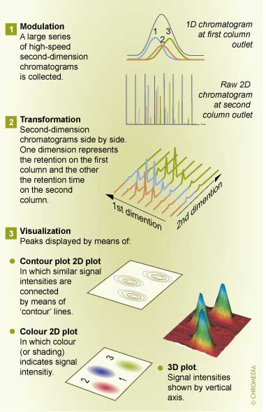
LC×LC systems can be easily constructed using conventional commercial high-pressure liquid chromatographic (HPLC) setups equipped with extra pump(s) and column(s) and an automated switching valve. In practice, there are several instrumental setups for the LC×LC, but in most cases 8-port or 10-port switching valves have been used. Best results are obtained when the loop volume is clearly larger than the volume of the fraction being collected. For example, if the fraction volume is 100 ml, an appropriate loop size is 125 to 150 ml.
There are two approaches that should be tested first, namely symmetrical and asymmetrical configuration, as shown in figure below. Both use either an 8-port or 10-port valve.
a. Symmetrical configuration. The flow direction is the same for both loops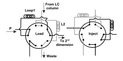
In asymmetrical configurations (Fig. b), each loop is flushed in a different direction into the second dimension.
b. Asymmetrical configuration.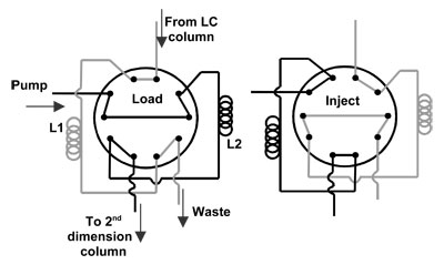
The figures show symmetrical and asymmetrical configurations of a switching valve displayed in both ![]() positions. L1 – loop 1; L2 – loop 2; LC – from the first dimension pump; P – from the second dimension pump; SEC – to the second-dimension column. The symmetrical configuration allows flushing of the fractions to the second dimensions in the same direction in which they were loaded, and thus making both positions identical.
positions. L1 – loop 1; L2 – loop 2; LC – from the first dimension pump; P – from the second dimension pump; SEC – to the second-dimension column. The symmetrical configuration allows flushing of the fractions to the second dimensions in the same direction in which they were loaded, and thus making both positions identical.
There also more complex solutions to be used. A modification of the sampling loop interface is the use of two guard columns instead of loops. The effluent from the first column is alternately trapped and sampled onto the secondary columns through a guard column interface. When one guard column traps the eluate, the other injects the previously trapped components onto a secondary column. This cycle is repeated throughout the analysis. The guard column is of the same material as the second-dimension column. A similar approach, utilizing 18 solid-phase extraction (SPE) columns, has also been developed. In this system, the use of several SPE columns allowed longer times for second-dimension separation without compromises in sampling frequency.
It is also possible to use two second-dimension columns connected in parallel or even use two modulator valves with two second-dimension columns. Also a stopped-flow approach utilizing two 6-port valves has been developed.The same MS systems that are used in conventional 1D LC-MS can be used also in LC×LC-MS. However, there are a few additional points that must be considered in the combination of LC×LC with MS:
1. Because the second-dimension eluent must be compatible with the MS some LC×LC combinations are not suitable with MS detection, for example, ion-exchange chromatography is not the best option for the second dimension separation.
2. Since the second-dimension separation in LC×LC is typically very rapid and the peak widths can be only a few seconds, the MS instrument must be capable of rapid detection. The minimum scanning rate of MS is about 5 Hz. Commercial TOF instruments are available with scanning rates as high as 200 scans/s, and are thus a good choice for LCxLC. Commercial single quadrupole instruments with high scanning rates have also recently become available and these can be used in LCxLC. However, triple quadrupole and ion-trap type analyzers are currently too slow for most LCxLC applications.
3. The second dimension separation should be preferably less than ca. 120 sec and this can be achieved by using high flow rates in the second dimension separation, up to several ml/min. Since the performances of many MS instruments suffer from high flow rates and the typically recommended flow rates are clearly lower (up to 1 ml/min), it is often necessary to use flow-splitting.