Abstract This chapter deals with the strategy that should be employed to transfer a gradient elution method from a given instrument and given column dimensions to a different instrument and/or different column dimensions. The different parameters affecting the gradient separation include the instrument dwell volume, the column length and the particle diameter. Simple rules are given to avoid change in the quality of the gradient separation while modifying these parameters. The problem of extra column volumes which may lead to additional extra column dispersion is pointed out. An interactive simulated gradient separation is put forward to help for a better understanding of these transfer rules.
LevelAdvanced
Transfer of gradient methods in dependence of operational parameters
An HPLC method is transferred when the instrument, the column dimensions and/or the flow-rate are changed. Transferring an optimized gradient elution method between different models (brands) of HPLC instruments and/or different column dimensions is less straightforward than transferring an optimized isocratic method. The gradient transfer is successful when first the selectivity of the gradient separation is not changed and second the peak band broadening is not affected by additional external dispersion.
Development of a gradient method:After having chosen the stationary phase and the solvents, the development of a gradient method should include four different steps:
- The extra-column dispersions are minimized and compared to the column dispersion so that their contribution to the total peak dispersion is insignificant.
- The good working of the gradient instrument is checked and the dwell
 volume is measured.
 - The gradient parameters are optimized.
- The gradient method is accurately described. This step is essential since a good transfer is impossible when the gradient method has not been fully described.
Transfer of a gradient method:
The transfer of the method also includes different steps. The first two steps are the same as those required for the method development. The third step consists in applying some simple rules of transfer. The vast majority of separations under gradient conditions are performed in reversed phase liquid chromatography (RPLC). The following discussion will therefore principally deal with reversed phase gradients. However the following given rules could also be applied to some extent to other HPLC methods (normal-phase, ion exchange, etc...).
Here, the different steps, except the one corresponding to the gradient optimization will be detailed and discussed through some illustrative examples.
Determination of extra–column variance, σ²ext, is a simple measurement which consists in replacing the column with a zero dead volume union and calculating the peak variance of a compound injected in usual conditions.
The extra-column variance has to be lower than 10% of the observed peak variance. For a Gaussian peak, the observed peak variance can be calculated from the measure of peak width at half peak height by ![]() (1)
(1)
Assuming that the different contributions to peak variance are independent, the observed peak variance is the sum of the following contributions:
![]() (2)
(2)
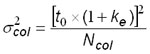
Were σ²col is the column peak variance which can be related to the column plate number Ncol for a compound having a retention factor at the point of elution, ke with
 (3)
(3)
With a linear gradient elution, ke values are similar for all solutes and typically within a range 1 to 5.
Eq.2 can be rewritten:
![]() (4)
(4)
By considering Eq.4, it clearly appears that minimizing the ratio σ2ext /σ2col is essential. A high value will affect all the peaks in a gradient separation.
The extra-column variance strongly depends on the extra-column volumes (injection, tubing and detection cell). It also depends on the time constant of the detector; especially in case of very fast separations with a small peak width value expressed in ![]() time unit
time unit
Checking the gradient system and determination of dwell volume, VD, can be performed simultaneously (Figure 1) by using methanol for the A-solvent and methanol with 0.05% acetone for the B-solvent, replacing the column with a zero-dead volume tubing and running a 0-100% B gradient in 20xt0.
Fig1: Dwell volume measurement. See text for explanation.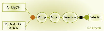
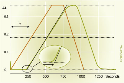 Figure 1: Dwell volume measurement. See text for explanation
The input gradient and the data system output are drawn in red and green respectively. The data system output is usually curved as shown in Figure 1. The dwell time, tD, should therefore be determined by measuring the intercept between the tangent to the gradient curve and the baseline. The dwell volume is obtained by multiplying the dwell time by the flow-rate.
This simple experiment is also very useful to check if the gradient system works correctly.
For a simple linear gradient elution, the gradient parameters usually include the initial composition, φi, the final composition, φf and the gradient time, TG, the gradient slope being given by (φf - φi)/TG. In addition to these parameters, the description of the method should include the time required to return to the initial composition and the time required to equilibrate the column. This latter is often expressed as a multiple of the column ![]() dead time, x.t0. The description of the method may also include a possible initial isocratic hold, tiso,i and a possible final isocratic hold, tiso,f. However, the initial isocratic hold never corresponds to the total delay time, tdelay, required for the gradient to reach the head of the column. This latter is given by
dead time, x.t0. The description of the method may also include a possible initial isocratic hold, tiso,i and a possible final isocratic hold, tiso,f. However, the initial isocratic hold never corresponds to the total delay time, tdelay, required for the gradient to reach the head of the column. This latter is given by
![]() (5)
(5)
The delay time should be known exactly and maintained identical when transferring the method. An additional time equal to the column dead time, t0, is required for the gradient to reach the detector cell. Here, the volume of the tube between the column outlet and the detector will be considered as insignificant.
These different parameters are illustrated in Figure 2 with a simulated gradient separation. Here, the time required to return to the initial composition is not considered. The gradient profiles at the point at which the mobile phase solvents are mixed (red point), at the column inlet (black point) and in the detector cell (blue point) are represented in red, black and blue respectively.
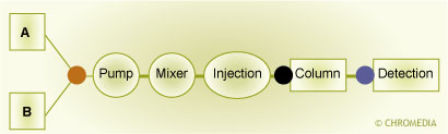
Fig 2: Gradient profiles at different points of the instrument.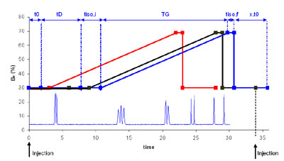 (The y-axis represents the composition of the mobile phase)
Some major conclusions can be drawn from Figure 2:
- The elution composition (represented in blue on figure 2) is the relevant composition to be considered when developing gradient methods. It is related to the retention time with
 (6)
(6) - The initial isocratic hold should be adjusted depending on the dwell time so that the total delay time is kept constant.
- The red gradient profile represents the mobile phase composition at the point at which the solvents are mixed and therefore it represents the gradient programming. As it can be seen on the figure, a time equal to the dwell time has to be added to the required equilibration time before the next injection otherwise the mobile phase composition at the column inlet (represented in black on the figure) could be different from the expected one. Hence, in the particular case of Fig. 2, the composition at the column inlet would be the final composition if a time corresponding to the dwell time is not added at the end of the gradient programming.
| Action | Time | % solvent B |
| Injection + gradient starting | 0 | φi |
| | tiso,i=tdelay-tD | φi |
| | tG+ tiso,i | φf |
| | tiso,f+ TG+ tiso,i | φf |
| | tiso,f+ TG+ tiso,i | φi |
| injection | x.t0+tD+tiso,f+ TG+ tiso,i | φi |
Alternatively, the dwell time can be set to zero by injecting the sample after the gradient has ![]() started. In this case the gradient programming becomes:
started. In this case the gradient programming becomes:
| Action | Time | % solvent B |
| gradient starting | -tD | φi |
| injection | 0 | φi |
| | tiso,i=tdelay | φi |
| | tG+ tiso,i | φf |
| | tiso,f+ TG+ tiso,i | φf |
| | tiso,f+ TG+ tiso,i | φi |
| gradient starting | x.t0 +tiso,f+ TG+ tiso,i | φi |
| injection | tD+x.t0+ tiso,f+ TG+ tiso,i | φi |
The transfer will be successful if the quality of the separation can just be affected by a possibly change in the column plate number due to a deliberate change in either column length or flow-rate. The quality of the separation between two adjacent peaks with a σobs, assumed to be more or less equal for both peaks, can be described by the resolution equation: ![]() (7)
(7)
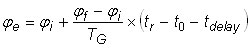
For a given pair of solutes and given initial and final compositions and according to the equations given in the appendix, the resolution is affected by the variation of three different parameters. When these parameters are kept constant the transfer is successfull.
Three rules for transferring a gradient.(Click to enlarge)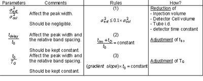
The following examples are illustrated by an attached simulated sheet representing two simulated separations. This interactive simulation is a tool which should allow to handle the transfer rules in various practical situations. Four examples are offered. However the user can change any parameter to see the effect on a gradient separation and better understand how the gradient works. Each example can be activated by clicking on the corresponding command button. Two chromatograms are presented. The blue one represents a gradient separation obtained in the laboratory which developed the method. The yellow one is a gradient separation obtained in the laboratory which received the method and had to adapt the gradient conditions. Depending on the conditions of transfer, the gradient time, the initial isocratic hold and/or the instrumental conditions have to be modified, according to the above ![]() rules, in order to keep the same resolution of all the components.
rules, in order to keep the same resolution of all the components.
Interactive tool to understand the transfer rules. (Click to download file, this is a large Excel file and may take a minute). Restricted to members. 
First example - Effect of the dwell volume
The dwell volume is frequently ignored by chromatographers when developing and/or transferring gradient methods. Therefore they are often replaced by isocratic ones to avoid difficulties. This first example shows the effect of the delay time on both retention and resolution. The transferring laboratory developed the method without isocratic hold and with a 4 mL dwell volume while the receiving laboratory used an instrument with a 1 mL dwell volume. Two major effects can be observed: first, a shift in retention which prevents from recognizing the peaks within a preset retention time window; second a loss in resolution for the less retained compounds. According to the second rule, one must adjust the delay time by introducing an isocratic hold (3mL).
Second example - Effect of the flow-rate
In this second example, the particle diameter was decreased and the flow-rate was therefore increased in order to work with a linear velocity close to the optimum as it can be seen on the Van Deemter curves. As shown on the simulated file, the quality of the separation is severely affected. According to the third rule, the quality of the separation can be maintained by keeping gradient slope x t0 constant, namely with tG=11.1 min. In this case, the ratio tdelay/t0 has not changed.
Third example - Effect of the column length
The particle diameter and the flow-rate are the same as in the preceding example but the column length is reduced to 12 cm. The column plate number is then the same for both chromatograms. In contrast, both tdelay/t0 and gradient slope x t0 are altered. As it can be seen, these modifications lead to a dramatic loss in resolution. The gradient method can be successfully transferred by varying TG (8.9 min) and by adding an isocratic hold (1.2 min). It is interesting to notice that both separations are then identical except that the analysis time of the yellow chromatogram is significantly lower (11.5 min instead of 26 min).
Fourth example – Effect of Transfer from HPLC to UPLC
This last example highlights the advantage of the use of smaller particles and the need of transfer rules to achieve a good transfer. From the transferring laboratory (HPLC method) to the receiving laboratory (UPLC method), many parameters were modified: the particle diameter (5µm to 1.7 µm), the column i.d. (4.6 mm to 2.1 mm), the column length (150 mm to 50 mm), the flow-rate (1 mL/min to 0.5 mL/min) and the dwell volume (4 mL to 0.1 mL). As it can be seen, tdelay/t0 and gradient slope x t0 are quite different. Furthermore, the external variance is highly reduced.
First the transfer rules must be applied to adjust TG (2.8 min) and tiso (0.4 min).
It clearly shows that these modifications are not enough to achieve a good separation. The HPLC instrumental conditions are not suitable for UPLC methods because the contribution of external dispersions to the peak band broadening is very much significant. The external volumes have therefore to be significantly reduced. The conditions to be changed include the cell volume (8µL to 0.5µL), the tube i.d. (0.25mm to 0.127mm) and the time constant of the detector (0.5s to 0.05s). The effect of each of these modifications on the peak width can be assessed on the yellow chromatogram. However, these changes are still not enough. A last concern exists about the solvent of injection. In the transferring laboratory, it was 70% ACN. Such a high solvent strength is not detrimental provided that the injection volume (5µL) is low compared to the column dead volume which is the case in the transferring laboratory. However it is highly detrimental with the UPLC method, especially for the less retained compounds. As a result, the sample has to be injected either in the initial mobile phase (30% ACN) or better in a solvent with a lower eluent strength (<30%ACN). Alternatively the injection volume should be decreased.
In case of a multilinear gradient elution, in addition to tiso,i and φi the gradient parameters include the successive compositions, φj and gradient times, TG,j (or isocratic holds tiso,j) corresponding to the different linear steps. As a result the transfer will be successful when on the one hand the two first rules in the above table are applied and on the other hand, the successive t0/TG,j and tiso,j/t0 are kept constant. This is illustrated in Figure 3 for a multilinear gradient separation of PTC-amino acids on two columns with different lengths. Both separations are identical except that the bottom separation is faster due to the reduction of column length. The effect of the associated decrease in column plate number is not noticeable.
Amino acid separation with multilinear gradient (click to enlarge)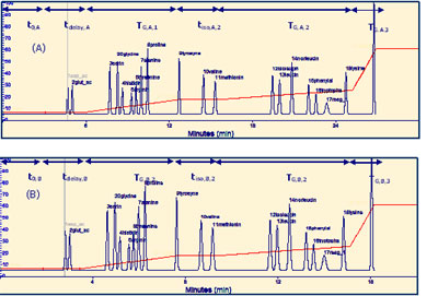 Figure 3 : Separation of PTC-amino acids with a multilinear gradient elution on columns with two different length. (A, top) 25 cm; (B, bottom) 15 cm. The acetonitrile content in the mobile phase is given on the Y-axis. The red gradient profile corresponds to the elution composition. The separation is recalculated using Osiris software.
Solution to the fundamental gradient equation according to the LSS theory. Click here to view the details of this theory.